9.2: Explainable models

Explainable models have inherent attributes that explain the impact that each feature has as weights or by creating a tree structure to explain the hierarchy of relationships amongst different features. The most prominent explainable models are linear regression, logistic regression, and decision trees.

9.2.1 Linear Regression

The linear regression models can explain at an overall level, the importance of each feature through the beta coefficient.

Its functional form is Y = ₀+ ₁x₁ + .. + _nx_n

Y is the predicted value of the dependent or outcome variable. ₀ is a constant term, ₁is the weight of the first feature x1 and _nis the weight of the nth feature x_n. If features are standardized and on the same scale, we can make comparisons amongst features to identify the most and least impactful features. In addition to this, through adjusted R², we can ascertain to what extent the model is better than a simple horizontal line through the mean value of the dependent variable.

By changing the value in each feature, we can observe the impact on the prediction outcome. Predictions are the sum product of weights and feature values. For numerical features, values can be increased or decreased. Categorical features can be represented as binary encoded 1 or 0 dummy features and the effect of their presence or absence can be compared with the model outcome. Modeling fashion clothing involvement ^[1] as the outcome, we can make inferences from table 9.2.1.

Table 9.2.1 Regression output for fashion clothing involvement

Although the model didn't explain all the variance in the data as evident from a low R square, it did however indicate that normative behavior is the biggest predictor of fashion clothing involvement. Normative influences are defined as the degree to which people conform to the expectations of society. Apart from this, age is negatively associated with fashion clothing involvement. Young people tend to be more involved in fashion clothing than those who are old. To a certain extent, married people are more fashionable than those who are unmarried.

9.2.2 Logistic Regression

The logistic regression follows the sigmoid function, which takes values between 0 and 1. 1 is the desired outcome. In total, the odds of events happening and not happening is 1. The cut-off is 0.5, this is otherwise known as the decision boundary.

Its functional form is

Where is a linear regression function and is equal to ₀+ ₁x₁ + .. + _nx_n

Predictions are probability values. For numerical features, values can be increased or decreased. Categorical features can be represented as binary encoded 1 or 0 dummy features. The effect of change in numerical and categorical dummy binary features on the outcome variable can be observed through the change in the position of the predicted outcome for the decision boundary.

For example, if for the baseline case the predicted outcome is 0.4 and after changing the value in features predicted outcome is 0.55, we can infer that the predicted class has changed from 0 to 1. For the value 0.4, as per the decision boundary of 0.5, it will be reduced to 0 as the outcome and for the predicted value of 0.55, it will be changed to 1.

The coefficients returned by logistic regression for each feature are the log of odds. Mathematically, it can be represented as a log (probability of event / (1-probability of the event)). Before interpreting the coefficients of the logistic regression beta coefficient, we need to convert the log of odds into the interpretable format. This can be done by first converting the log into the exponential form using the formula odd = exponential (original form log of odd). Finally, by doing odds/(1 + odds), we can compare the coefficients of each feature if they are all standardized.

We can analyze the psychological impact of COVID-19 among primary healthcare workers through logistic regression from the below logistic regression output ^[2]. Table 9.2.2 has output from the logistic regression model.

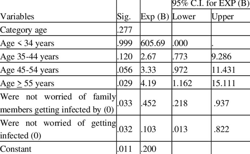
Table 9.2.2 Regression output for psychological impact of COVID-19 among primary healthcare workers

Older healthcare workers "55 years or older" were four times more vulnerable to depression than younger workers. Healthcare workers who were neither worried for themselves nor for their families were found to be less likely to have depression disorder in comparison to those who worried for themselves and their families.

In the case of text classification, we can obtain logistic regression weights for each corresponding word feature. This will help us explain the relative importance of each word.

9.2.3 Decision Tree

The decision trees can be trained to identify different classes for a classification problem. It can also be trained for a regression problem. Training the decision tree is otherwise called growing a decision tree. It is performed through a splitting process. Adding a section to a tree is called grafting whereas cutting a tree or its node is called pruning. The dependent variable is split with the help of independent variables at nodes with the most optimal value into branches based on the best split. The best split is decided based on either of the methods such as the Gini index, information gain, or chi-square.

CART (Classification and Regression Trees) uses Gini as the method to evaluate split into data. For a pure population, the score is 0. This is most useful in noisy data. If the dependent variable has n number of classes, for each feature, the Gini impurity is calculated and the one with the lowest impurity is chosen. In the case of information gain or entropy, after calculating the information gain for each feature, the one with the highest is selected for the node splitting.

For numerical features, exclusion points are selected and values less than and higher than the exclusion point are encoded as ordinal levels. This makes the feature binary. Through n possible exclusion points, the one which gives maximum information gain or minimum Gini impurity is selected.

A study for potential diabetes mellitus created a decision tree to model potential risk for diabetes based on diet, lifestyle, and past family history of diabetes ^[3]. Figure 9.2.3 has the decision tree diagram.

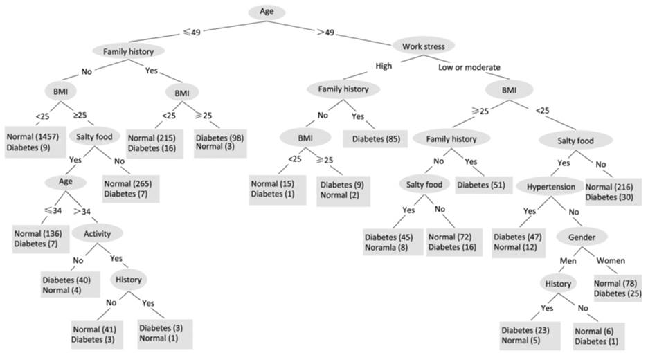
Figure 9.2.3 Potential risk for diabetes using decision tree

If we traverse from top to bottom of the decision tree across 'nodes', data is automatically filtered as a subset based on the 'and' condition. For example, let's traverse the right edge of the tree as Age(>40) -> Work Stress(High) -> Family History(Yes) -> Diabetes(85). The node and edges can be translated as people with age above 40 and who also have high work stress and family history of other family members having been diagnosed with diabetes, it is certain that the person will have diabetes. All the 85 observations falling under this group are diagnosed with diabetes.

We can scale the Gini index or entropy at each node so that it adds to 100. It can help us compare between different subsets of data created with decision tree "AND" rules. We can narrow down to identify the most and least impactful subsets of data and rules affecting the dependent variable.