10.4: Feature Extraction

In the case of text classification, feature extraction is done by representing text documents into matrices, which can then be used by machine learning algorithms as features to classify labels. For traditional machine learning models, feature extraction is done mostly by either a bag of words matrix or the TF-IDF matrix.

10.4.1  Bag of Words

It is a scoring method in which the count of individual words is used for presence and 0 for absence. Let us consider example 10.4.1 below with 4 corpora.

Example 10.4.1

Corpus 1: I am very happy.

Corpus 2: I just had an awesome weekend.

Corpus 3: I just had lunch. You had lunch?

Corpus 4: Do you want chips?

Unique words from these 4 corpora, after removing punctuation marks are: 'am', 'an', 'awesome', 'chips', 'Do', 'had', 'happy', 'I', 'just', 'lunch', 'very', 'want', 'weekend', 'you'

Bag of words vector will appear in table 10.4.1.

Table 10.4.1: Bag of words vector

In the above table, the corpus is present in the column and the words are present in the row. If a specific word is present in the corpus, its count is presented in corresponding cells against the word. If a word is not present in the corpus, 0 is presented in the corresponding cell.

For example, the word  lunch  is present in corpus 3. Hence count 2 is present in the corresponding cell. The word  am  is only present in corpus 1, for once. Hence the corresponding cells have the value 1. Again, the word  am , is not present in any other corpus apart from corpus 1. Hence, in corpus 2, 3, and 4, the value in the corresponding cells is 0.

10.4.2  Term Frequency Inverse Document Frequency

This is otherwise abbreviated as TF-IDF. Term frequency and inverse document frequency of each word are calculated and multiplied to obtain the TF-IDF score.

Term frequency (TF) is calculated by dividing how frequently a term appears in a corpus, by the total number of terms in the corpus.

TF = Count of the number of times the term  t  is present in the corpus) / Count all the terms in the corpus.

Inverse document frequency is calculated by taking the logarithm of the total number of the corpus by the count of documents that has the term.

IDF = log (Total number of documents / Count(documents which have term  t ))

TF-IDF vector for the corpora in example 10.4.1 will appear as per table 10.4.2

Table 10.4.2: TF-IDF vector

10.4.3  Word2vec

Word2Vec is a shallow neural network that tries to understand the context of words ^[10]. In word2vec, individual words are represented as one-hot vectors and are used for creating a vector space. It has a hidden layer, which is a fully-connected dense layer. The weights of the hidden layer are the word embeddings. The output layer outputs probabilities based on the Softmax activation function for the target words from the vocabulary. Such a network is a "standard" multinomial (multi-class) classifier.

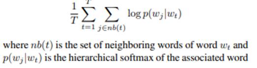
The objective function of word2vec is to maximize the log of similarity between the vectors for words that appear close together in the context and minimize the similarity of words that do not. This is called the Softmax function.

Since classes are actual words, the number of neurons is huge. The Softmax function when applied to such a huge output layer will be computationally expensive. To save costly computation of the Softmax in the output layer, noise-contrastive estimation is used. This converts the multinomial classification problem to a binary classification problem.

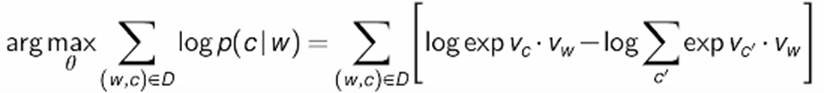
C is the context word, and W is the focus word. V_c is the embedding of context words and V_w is the embedding of focus words.

Given a pair of words, we will predict the context target or not. For this, we will create positive and negative samples. For example, if 'Orange' and 'juice' are positive, it will be inferred that these appear together in the same context. Similarly, if 'Orange', and 'king' are negative, it will be inferred that both words do not appear in the same context. Positive samples are extracted from the context window whereas negative sample is drawn randomly from the dictionary of all words. Depending on the size of the data, if the data is small, negative sample size k is selected between 5<>20 and for large, k is between 2<>5. Accordingly, word pairs are created consisting of the input word, surrounding context word, and target label whether it is a positive sample or negative sample.

For backpropagation, two matrices of the same size are created namely embedding and context. The number of rows in the matrix is the size of the vocabulary in the corpus and the number of columns is defined as the size of the embedding. The embedding matrix has input word representation and the context matrix has representation from context word. At the start of the training process, random values are initialized in these matrices.

Through the dot product of input embedding with each of the context embeddings, we obtain similarities between the input and context embeddings. Resultant dot product numbers are converted into positive numbers ranging between 0 and 1 using the sigmoid function. The prediction error is obtained for each pair of input words and context words by subtracting sigmoid transformation from the actual label value of the positive sample(1) and negative sample(0). The error so obtained is inserted in the embedding layer for each of the words in input for all the combination pairs. This process is repeated through the dataset, based on the number of epochs defined. Finally, the context matrix is discarded and the embedding matrix is used.